Tidy Tuesday - Coffee Rating
Predicting Process of Green Coffee Beans
With coffee being a hobby of mine, I was scrolling through past Tidy Tuesdays and found one on coffee ratings. Originally I thought looking at predictions of total cup points, but I assumed with all the coffee tasting characteristics that it wouldn’t really tell me anything. Instead, I decided to look into the processing method, as there are different taste characteristics between washed and other processing methods.
coffee <- read_csv('https://raw.githubusercontent.com/rfordatascience/tidytuesday/master/data/2020/2020-07-07/coffee_ratings.csv') %>%
  mutate(species = as.factor(species),
         process = recode(processing_method, "Washed / Wet" = "washed",
                          "Semi-washed / Semi-pulped" = "not_washed",
                          "Pulped natural / honey" = "not_washed",
                          "Other" = "not_washed",
                          "Natural / Dry" = "not_washed",
                          "NA" = NA_character_),
         process = as.factor(process),
         process = relevel(process, ref = "washed"),
         country_of_origin = as.factor(country_of_origin)) %>%
  drop_na(process) %>%
  filter(country_of_origin != "Cote d?Ivoire")
##
## -- Column specification --------------------------------------------------------
## cols(
##   .default = col_character(),
##   total_cup_points = col_double(),
##   number_of_bags = col_double(),
##   aroma = col_double(),
##   flavor = col_double(),
##   aftertaste = col_double(),
##   acidity = col_double(),
##   body = col_double(),
##   balance = col_double(),
##   uniformity = col_double(),
##   clean_cup = col_double(),
##   sweetness = col_double(),
##   cupper_points = col_double(),
##   moisture = col_double(),
##   category_one_defects = col_double(),
##   quakers = col_double(),
##   category_two_defects = col_double(),
##   altitude_low_meters = col_double(),
##   altitude_high_meters = col_double(),
##   altitude_mean_meters = col_double()
## )
## i Use `spec()` for the full column specifications.
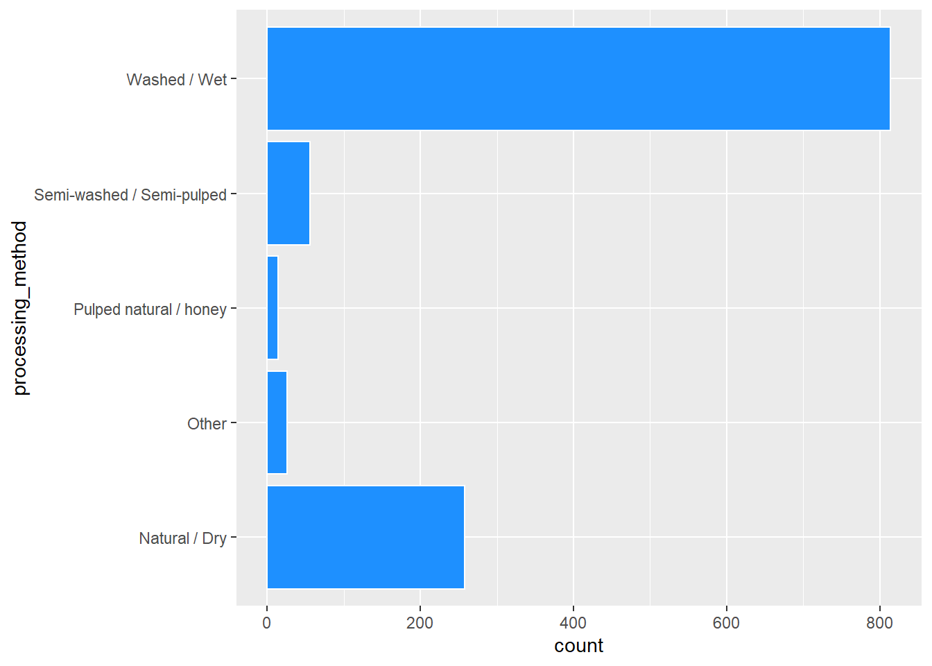
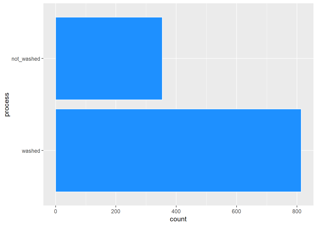
After looking at the distributions of procssing methods, I also decided to make the processing method binary with washed and not washed. This worked out better for the prediction models. There are also some descriptives of each variable.
coffee %>%
  ggplot(aes(processing_method)) +
  geom_bar(color = "white", fill = "dodgerblue") +
  coord_flip()
coffee %>%
  ggplot(aes(process)) +
  geom_bar(color = "white", fill = "dodgerblue") +
  coord_flip()
psych::describe(coffee, na.rm = TRUE)[c("n", "mean", "sd", "min", "max", "skew", "kurtosis")]
##                           n    mean      sd   min       max  skew kurtosis
## total_cup_points       1168   82.06    2.71 59.83     90.58 -1.95     9.26
## species*               1168    1.01    0.09  1.00      2.00 10.65   111.61
## owner*                 1161  133.43   76.78  1.00    287.00  0.10    -1.00
## country_of_origin*     1168   14.79   10.08  1.00     36.00  0.31    -1.12
## farm_name*              883  271.04  154.16  1.00    524.00  0.00    -1.27
## lot_number*             239   93.18   59.86  1.00    202.00  0.18    -1.27
## mill*                   931  196.60  122.71  1.00    419.00  0.24    -1.28
## ico_number*            1057  360.89  242.05  1.00    753.00  0.08    -1.27
## company*               1077  141.73   76.77  1.00    266.00 -0.10    -1.23
## altitude*              1014  154.54   98.40  1.00    351.00  0.32    -1.04
## region*                1137  174.91   87.74  1.00    325.00 -0.11    -1.09
## producer*               995  314.12  175.27  1.00    624.00 -0.04    -1.12
## number_of_bags         1168  153.80  130.08  1.00   1062.00  0.37     0.50
## bag_weight*            1168   23.50   16.67  1.00     45.00 -0.23    -1.71
## in_country_partner*    1168    9.68    7.04  1.00     25.00  0.41    -1.31
## harvest_year*          1161    5.82    2.95  1.00     14.00  0.76    -0.46
## grading_date*          1168  242.39  144.52  1.00    495.00  0.11    -1.21
## owner_1*               1161  135.29   77.68  1.00    290.00  0.09    -1.00
## variety*               1089   12.61    9.77  1.00     29.00  0.63    -1.24
## processing_method*     1168    3.98    1.67  1.00      5.00 -1.13    -0.62
## aroma                  1168    7.56    0.31  5.08      8.75 -0.55     4.46
## flavor                 1168    7.51    0.34  6.08      8.83 -0.34     1.73
## aftertaste             1168    7.39    0.34  6.17      8.67 -0.45     1.36
## acidity                1168    7.53    0.31  5.25      8.75 -0.30     3.31
## body                   1168    7.52    0.28  6.33      8.50 -0.10     0.89
## balance                1168    7.51    0.34  6.08      8.58 -0.10     1.17
## uniformity             1168    9.84    0.50  6.00     10.00 -4.21    20.83
## clean_cup              1168    9.84    0.75  0.00     10.00 -6.98    62.29
## sweetness              1168    9.89    0.52  1.33     10.00 -7.53    80.78
## cupper_points          1168    7.48    0.40  5.17      8.75 -0.64     2.79
## moisture               1168    0.09    0.05  0.00      0.17 -1.41     0.35
## category_one_defects   1168    0.51    2.70  0.00     63.00 14.43   279.42
## quakers                1167    0.17    0.82  0.00     11.00  6.87    57.30
## color*                 1070    2.80    0.64  1.00      4.00 -1.51     2.57
## category_two_defects   1168    3.79    5.54  0.00     55.00  3.54    18.53
## expiration*            1168  241.61  144.11  1.00    494.00  0.12    -1.21
## certification_body*    1168    9.38    6.65  1.00     24.00  0.37    -1.31
## certification_address* 1168   16.58    7.33  1.00     29.00 -0.19    -1.06
## certification_contact* 1168    9.39    7.26  1.00     26.00  0.36    -0.96
## unit_of_measurement*   1168    1.87    0.34  1.00      2.00 -2.21     2.87
## altitude_low_meters    1012 1796.86 9073.21  1.00 190164.00 19.36   384.12
## altitude_high_meters   1012 1834.27 9071.86  1.00 190164.00 19.36   384.03
## altitude_mean_meters   1012 1815.56 9072.31  1.00 190164.00 19.36   384.12
## process*               1168    1.30    0.46  1.00      2.00  0.86    -1.27
Now, its time to split the data into training and testing data. I also included the function of strata to stratify sampling based on process.
set.seed(05132021)

coffee_split <- initial_split(coffee, strata = "process")

coffee_train <- training(coffee_split)
coffee_test <- testing(coffee_split)
I also did some cross validation for the training dataset and used the metrics I was most interested in.
set.seed(05132021)

coffee_fold <- vfold_cv(coffee_train, strata = "process", v = 10)

metric_measure <- metric_set(accuracy, mn_log_loss, roc_auc)
From the beginning I was interested in the tasting characteristics and how they would predict whether the green coffee was washed or not washed. I also included the total cup points because I wanted to see the importance of that predictor on the processing method. The only feature engineering I did was to remove any zero variance in the predictors of the model.
set.seed(05132021)

char_recipe <- recipe(process ~ aroma + flavor + aftertaste +
                        acidity + body + balance + uniformity + clean_cup +
                        sweetness + total_cup_points,
                      data = coffee_train) %>%
  step_zv(all_predictors(), -all_outcomes())

char_recipe %>%
  prep() %>%
  bake(new_data = NULL) %>%
  head()
## # A tibble: 6 x 11
##   aroma flavor aftertaste acidity  body balance uniformity clean_cup sweetness
##   <dbl>  <dbl>      <dbl>   <dbl> <dbl>   <dbl>      <dbl>     <dbl>     <dbl>
## 1  8.17   8.58       8.42    8.42  8.5     8.25         10        10        10
## 2  8.08   8.58       8.5     8.5   7.67    8.42         10        10        10
## 3  8.17   8.17       8       8.17  8.08    8.33         10        10        10
## 4  8.42   8.17       7.92    8.17  8.33    8            10        10        10
## 5  8.5    8.5        8       8     8       8            10        10        10
## 6  8      8          8       8.25  8       8.17         10        10        10
## # ... with 2 more variables: total_cup_points <dbl>, process <fct>
Logistic Regression
The first model I wanted to test with the current recipe was logistic regression. The accuracy and roc auc were alright for a starting model.
## Warning: package 'rlang' was built under R version 4.0.4
collect_metrics(lr_fit)
## # A tibble: 3 x 6
##   .metric     .estimator  mean     n std_err .config
##   <chr>       <chr>      <dbl> <int>   <dbl> <chr>
## 1 accuracy    binary     0.698    10 0.00342 Preprocessor1_Model1
## 2 mn_log_loss binary     0.589    10 0.00775 Preprocessor1_Model1
## 3 roc_auc     binary     0.648    10 0.0188  Preprocessor1_Model1
Lasso Regression
Now for the first penalized regression. The lasso regression did not improve in either metric. Let’s try the next penalized regression.
collect_metrics(lasso_fit)
## # A tibble: 3 x 6
##   .metric     .estimator  mean     n std_err .config
##   <chr>       <chr>      <dbl> <int>   <dbl> <chr>
## 1 accuracy    binary     0.702    10 0.00397 Preprocessor1_Model1
## 2 mn_log_loss binary     0.592    10 0.00850 Preprocessor1_Model1
## 3 roc_auc     binary     0.645    10 0.0191  Preprocessor1_Model1
Ridge Regression
The ridge regression was shown to not be a good fitting model. So I tested an additional penalized regression while tuning hyper-parameters.
collect_metrics(ridge_fit)
Elastic Net Regression
The elastic net regression had slightly better accuracy than the non-penalized logistic regression but the ROC AUC was exactly the same. While the elastic net regression did not take long computationally due to the small amount of data, this model would not be chosen over the logistic regression.
collect_metrics(elastic_fit)
## # A tibble: 300 x 8
##        penalty mixture .metric    .estimator  mean     n std_err .config
##          <dbl>   <dbl> <chr>      <chr>      <dbl> <int>   <dbl> <chr>
##  1    1   e-10       0 accuracy   binary     0.698    10 0.00342 Preprocessor1_~
##  2    1   e-10       0 mn_log_lo~ binary     0.589    10 0.00775 Preprocessor1_~
##  3    1   e-10       0 roc_auc    binary     0.648    10 0.0188  Preprocessor1_~
##  4    1.29e- 9       0 accuracy   binary     0.698    10 0.00342 Preprocessor1_~
##  5    1.29e- 9       0 mn_log_lo~ binary     0.589    10 0.00775 Preprocessor1_~
##  6    1.29e- 9       0 roc_auc    binary     0.648    10 0.0188  Preprocessor1_~
##  7    1.67e- 8       0 accuracy   binary     0.698    10 0.00342 Preprocessor1_~
##  8    1.67e- 8       0 mn_log_lo~ binary     0.589    10 0.00775 Preprocessor1_~
##  9    1.67e- 8       0 roc_auc    binary     0.648    10 0.0188  Preprocessor1_~
## 10    2.15e- 7       0 accuracy   binary     0.698    10 0.00342 Preprocessor1_~
## # ... with 290 more rows
show_best(elastic_fit, metric = "accuracy", n = 5)
## # A tibble: 5 x 8
##        penalty mixture .metric  .estimator  mean     n std_err .config
##          <dbl>   <dbl> <chr>    <chr>      <dbl> <int>   <dbl> <chr>
## 1     7.74e- 2   0.111 accuracy binary     0.703    10 0.00434 Preprocessor1_Mo~
## 2     1   e-10   0.333 accuracy binary     0.703    10 0.00422 Preprocessor1_Mo~
## 3     1.29e- 9   0.333 accuracy binary     0.703    10 0.00422 Preprocessor1_Mo~
## 4     1.67e- 8   0.333 accuracy binary     0.703    10 0.00422 Preprocessor1_Mo~
## 5     2.15e- 7   0.333 accuracy binary     0.703    10 0.00422 Preprocessor1_Mo~
show_best(elastic_fit, metric = "roc_auc", n = 5)
## # A tibble: 5 x 8
##        penalty mixture .metric .estimator  mean     n std_err .config
##          <dbl>   <dbl> <chr>   <chr>      <dbl> <int>   <dbl> <chr>
## 1     1   e-10       0 roc_auc binary     0.648    10  0.0188 Preprocessor1_Mod~
## 2     1.29e- 9       0 roc_auc binary     0.648    10  0.0188 Preprocessor1_Mod~
## 3     1.67e- 8       0 roc_auc binary     0.648    10  0.0188 Preprocessor1_Mod~
## 4     2.15e- 7       0 roc_auc binary     0.648    10  0.0188 Preprocessor1_Mod~
## 5     2.78e- 6       0 roc_auc binary     0.648    10  0.0188 Preprocessor1_Mod~
select_best(elastic_fit, metric = "accuracy")
## # A tibble: 1 x 3
##   penalty mixture .config
##     <dbl>   <dbl> <chr>
## 1  0.0774   0.111 Preprocessor1_Model019
select_best(elastic_fit, metric = "roc_auc")
## # A tibble: 1 x 3
##        penalty mixture .config
##          <dbl>   <dbl> <chr>
## 1 0.0000000001       0 Preprocessor1_Model001
New Recipe
Even though the elastic net regression was only slightly better, I decided to update the workflow using that model. This time I decided to update the recipe by including additional predictors like if there were any defects in the green coffee beans, the species of the coffee (e.g., Robusta and Arabica), and the country of origin. I also included additional steps in my recipe by transforming the category predictors and working with the factor predictors, like species, and country of origin. The inclusion of additional steps and the predictors created a better fitting model with the elastic net regression.
set.seed(05132021)

bal_rec <- recipe(process ~ aroma + flavor + aftertaste +
                        acidity + body + balance + uniformity + clean_cup +
                        sweetness + total_cup_points + category_one_defects + category_two_defects + species +
                        country_of_origin,
                      data = coffee_train) %>%
  step_BoxCox(category_two_defects, category_one_defects) %>%
  step_novel(species, country_of_origin) %>%
  step_other(species, country_of_origin, threshold = .01) %>%
  step_unknown(species, country_of_origin) %>%
  step_dummy(species, country_of_origin) %>%
  step_zv(all_predictors(), -all_outcomes())
collect_metrics(elastic_bal_fit)
## # A tibble: 300 x 8
##        penalty mixture .metric    .estimator  mean     n std_err .config
##          <dbl>   <dbl> <chr>      <chr>      <dbl> <int>   <dbl> <chr>
##  1    1   e-10       0 accuracy   binary     0.839    10 0.00923 Preprocessor1_~
##  2    1   e-10       0 mn_log_lo~ binary     0.431    10 0.0153  Preprocessor1_~
##  3    1   e-10       0 roc_auc    binary     0.840    10 0.0163  Preprocessor1_~
##  4    1.29e- 9       0 accuracy   binary     0.839    10 0.00923 Preprocessor1_~
##  5    1.29e- 9       0 mn_log_lo~ binary     0.431    10 0.0153  Preprocessor1_~
##  6    1.29e- 9       0 roc_auc    binary     0.840    10 0.0163  Preprocessor1_~
##  7    1.67e- 8       0 accuracy   binary     0.839    10 0.00923 Preprocessor1_~
##  8    1.67e- 8       0 mn_log_lo~ binary     0.431    10 0.0153  Preprocessor1_~
##  9    1.67e- 8       0 roc_auc    binary     0.840    10 0.0163  Preprocessor1_~
## 10    2.15e- 7       0 accuracy   binary     0.839    10 0.00923 Preprocessor1_~
## # ... with 290 more rows
show_best(elastic_bal_fit, metric = "accuracy", n = 5)
## # A tibble: 5 x 8
##    penalty mixture .metric  .estimator  mean     n std_err .config
##      <dbl>   <dbl> <chr>    <chr>      <dbl> <int>   <dbl> <chr>
## 1 0.000464   0.111 accuracy binary     0.840    10 0.0101  Preprocessor1_Model0~
## 2 0.000464   0.222 accuracy binary     0.840    10 0.0101  Preprocessor1_Model0~
## 3 0.00599    0.111 accuracy binary     0.840    10 0.00933 Preprocessor1_Model0~
## 4 0.00599    0.222 accuracy binary     0.840    10 0.00933 Preprocessor1_Model0~
## 5 0.00599    0.333 accuracy binary     0.840    10 0.00933 Preprocessor1_Model0~
show_best(elastic_bal_fit, metric = "mn_log_loss", n = 5)
## # A tibble: 5 x 8
##    penalty mixture .metric    .estimator  mean     n std_err .config
##      <dbl>   <dbl> <chr>      <chr>      <dbl> <int>   <dbl> <chr>
## 1 0.000464   1     mn_log_lo~ binary     0.420    10  0.0179 Preprocessor1_Mode~
## 2 0.000464   0.889 mn_log_lo~ binary     0.420    10  0.0178 Preprocessor1_Mode~
## 3 0.000464   0.778 mn_log_lo~ binary     0.420    10  0.0178 Preprocessor1_Mode~
## 4 0.000464   0.667 mn_log_lo~ binary     0.420    10  0.0178 Preprocessor1_Mode~
## 5 0.000464   0.556 mn_log_lo~ binary     0.420    10  0.0177 Preprocessor1_Mode~
show_best(elastic_bal_fit, metric = "roc_auc", n = 5)
## # A tibble: 5 x 8
##    penalty mixture .metric .estimator  mean     n std_err .config
##      <dbl>   <dbl> <chr>   <chr>      <dbl> <int>   <dbl> <chr>
## 1 0.00599    0.778 roc_auc binary     0.843    10  0.0150 Preprocessor1_Model078
## 2 0.000464   0.667 roc_auc binary     0.843    10  0.0141 Preprocessor1_Model067
## 3 0.00599    0.889 roc_auc binary     0.843    10  0.0148 Preprocessor1_Model088
## 4 0.000464   0.444 roc_auc binary     0.843    10  0.0141 Preprocessor1_Model047
## 5 0.000464   0.556 roc_auc binary     0.843    10  0.0141 Preprocessor1_Model057
select_best(elastic_bal_fit, metric = "accuracy")
## # A tibble: 1 x 3
##    penalty mixture .config
##      <dbl>   <dbl> <chr>
## 1 0.000464   0.111 Preprocessor1_Model017
select_best(elastic_bal_fit, metric = "mn_log_loss")
## # A tibble: 1 x 3
##    penalty mixture .config
##      <dbl>   <dbl> <chr>
## 1 0.000464       1 Preprocessor1_Model097
select_best(elastic_bal_fit, metric = "roc_auc")
## # A tibble: 1 x 3
##   penalty mixture .config
##     <dbl>   <dbl> <chr>
## 1 0.00599   0.778 Preprocessor1_Model078
Now using the testing dataset, we can see how well the final model fit the testing data. While not the best at predicting washed green coffee beans, this was a good test to show that the penalized regressions are not always the best fitting models compared to regular logistic regression. In the end, it seemed like the recipe was the most important component to predicting washed green coffee beans.
final_results %>%
  collect_metrics()
## # A tibble: 2 x 4
##   .metric  .estimator .estimate .config
##   <chr>    <chr>          <dbl> <chr>
## 1 accuracy binary         0.823 Preprocessor1_Model1
## 2 roc_auc  binary         0.817 Preprocessor1_Model1
Jonathan A. Pedroza (JP)
Lecturer in Psychology at Cal Poly Pomona
My research interests revolve around addressing health inequities in underrepresented populations.